An Easy-To-Follow Introduction To The CNOT Gate
It's time to learn about Multi-qubit quantum gates, starting with the CNOT gate.

We have learned a great deal about single-qubit quantum gates over the past few weeks.
It’s now time to start learning about multi-qubit quantum gates.
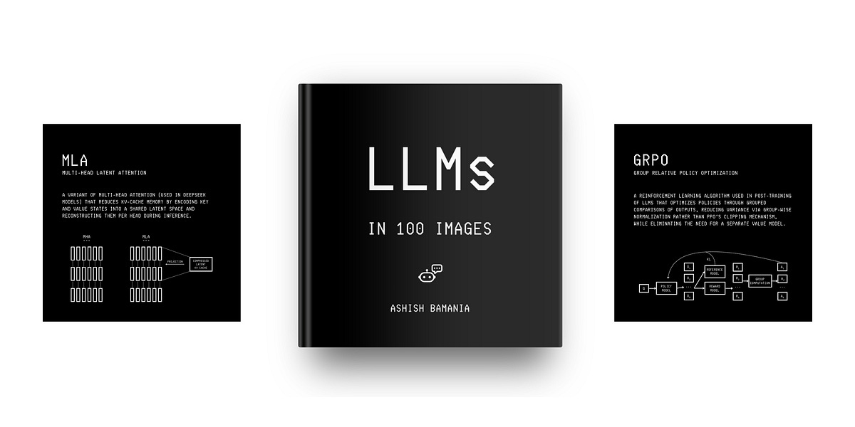
My latest book, called “LLMs In 100 Images”, is now out!
It is a collection of 100 easy-to-follow visuals that describe the most important concepts you need to master LLMs today.
Grab your copy today at a special early bird discount using this link.
What Are Multi-Qubit Quantum Gates?
Multi-qubit quantum gates are quantum logic gates that operate on two or more qubits simultaneously.
They are represented by 2ⁿ × 2ⁿ unitary matrices, where n is the number of qubits the gate acts upon.
Let’s go back a bit to understand how they work better.
We know from previous lessons that quantum states are unit vectors in 2ⁿ-dimensional complex space.
For example, a single qubit is represented by a unit vector in a two-dimensional complex space as a superposition of the computational basis states |0> and |1>.

where:

Similarly, a multi-qubit system of 2 qubits is represented by the tensor product of the constituent quantum states.
For the following two individual quantum states:

The combined 2-qubit state system is represented by their tensor product as follows:


These values correspond to the coefficients of the basis states |00>, |01>, |10> , and |11> respectively.
And their square represents the probability of measuring the multi-qubit system in the corresponding state.
For a gate to act on n qubits, it has to be a 2ⁿ × 2ⁿ unitary matrix.
For example, for a single qubit, a gate acting on it has to be a unitary matrix of dimension 2 x 2.
Similarly, for a 2-qubit system, a gate acting on it has to be a unitary matrix of dimension 2² x 2² or a 4 x 4 matrix.
Let’s move forward to learn about our first multi-qubit Quantum gate next.
The CNOT Gate
The CNOT gate, or Controlled-NOT gate, is a two-qubit gate.
It receives two inputs and gives out two outputs.
The first input is called the Control qubit, and the second one is called the Target qubit.
The CNOT gate flips the state of the target qubit only if the control qubit is in the state |1>. Otherwise, it does nothing to the target.
The control qubit is always returned unchanged as one of the outputs.
Take an example of the two qubits |A> and |B> as shown below:

When the CNOT gate is applied with |A> as the control qubit, and |B> as the target qubit, the outputs returned are:
Output 1 is
|1>(Control qubit|A>is returned unchanged.)Output 2 is
|1>(|B> = |0>is flipped as the control qubit|A>was|1>.)
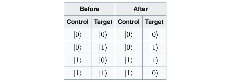
Truth Table
The truth table for the CNOT gate is as follows.
Circuit Symbol
In a quantum circuit, the CNOT is represented using the following symbol, where:
The ● symbol represents the control qubit.
The ⊕ symbol represents the target qubit and indicates that a NOT operation (Pauli-X) is applied to it conditionally.

Matrix Representation
The CNOT gate is represented by the following matrix:

Consider these two qubits |A> and |B> again:
The combined input state to the CNOT gate is as follows:

In a two-qubit system, the four computational basis states are |00>, |01>, |10>, and |11>.
On this basis:

When we apply the CNOT gate to it, the following matrix multiplication takes place:

The result is equal to the |11> .

Creating Entangled States With The CNOT Gate
One of the important applications of the CNOT gate is in creating maximally entangled two-qubit states, known as Bell states.
Consider the following, one of four Bell states:

It represents a quantum system where the measurement of one qubit instantaneously determines the state of the other, no matter how far apart they are.
If one qubit is measured and found to be in state |0>, the other will also be |0>. Otherwise, if one is found to be in state |1>, the other will also be |1>.
Even though the probability of obtaining a state from the first measurement is random (50% chance for |0>, and 50% for |1>), the two qubits always end up in the same state when one of them is measured.
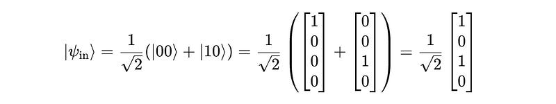
To create this Bell state |Φ+>, the CNOT gate is applied with:
The control qubit in the following superposition state:

The target qubit as
|0>
The resulting input state to the CNOT gate is:


When the CNOT gate is applied to this state:
For the first term
|00>, given the control qubit is|0>, the target qubit|0>does not change. The result is therefore|00>.For the second term
|10>, given the control qubit is|1>, the target qubit|0>changes to|1>. The result is therefore|11>.
The final state after applying the CNOT gate is:

We can confirm this with explicit matrix multiplication operations as follows.
The input to the gate is as follows:
The CNOT gate acts on this as follows:
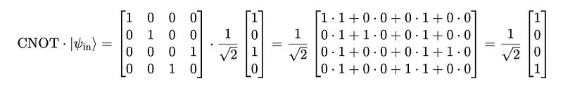
The final result is therefore:

This is the Bell state |Φ+>.
That’s a brief introduction to the CNOT gate. Stay tuned for upcoming lessons, where we will explore some more multi-qubit quantum gates!