All The Math That You Need To Start Doing Quantum Computing (Part 7)
Lesson 7: Linear Algebra (3) - Matrices


In this lesson, we further discuss concepts from Linear Algebra that are essential for learning about Quantum systems.
In case you missed the previous lessons on the mathematics required for quantum mechanics and quantum computing, here they are:
Lesson 7: Linear Algebra (3)
Matrices
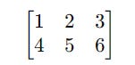
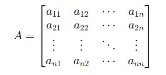
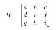
A Matrix is a rectangular array of numbers (elements).
A m x n matrix has m rows and n columns.
These are also called the dimensions of a matrix.
A matrix with the same number of rows and columns is called a Square matrix.
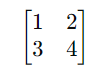
For square matrices, the main diagonal is the line of entries running from the top-left corner to the bottom-right corner.
It is also called the principal diagonal, primary diagonal, leading diagonal, or major diagonal.
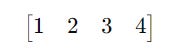
A bra can be seen as a matrix with just one row.
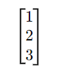
Similarly, a ket can be seen as a matrix with just one column.
In Quantum mechanics, matrices are used to:
describe the Quantum States using ket vectors or column matrices
create Quantum Gates, which are matrices that act to transform quantum states
Matrix Addition & Subtraction
Only matrices with the same dimensions can be added or subtracted.
For example, you can add/subtract a 2 x 2 matrix with/from another 2 x 2 matrix but cannot add/subtract a 2 x 2 matrix with/from a 3 x 2 matrix.
This is done element-wise, as shown below.
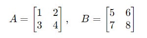
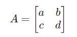
Consider two 2 x 2 matrices named A and B :
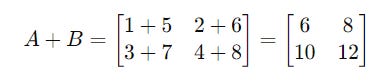
They are added as follows:
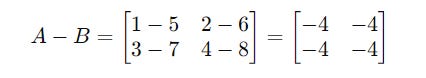
Similarly, they can be subtracted as follows:
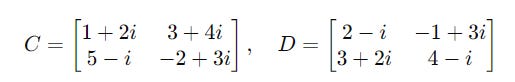
The rules apply similarly even when matrix elements are complex numbers.
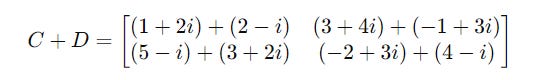
For two matrices C and D with complex numbers as their elements:
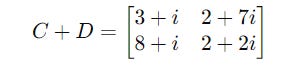
They are added as follows:
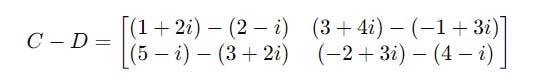
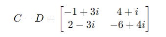
Similarly, they can be subtracted as follows:
Scalar Multiplication
Multiplying a matrix with a number (scaler) is simple.
It involves just multiplying each element in the matrix by the number.
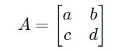
For a matrix A:
Multiplying it with a scalar k results in:
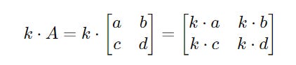
We can see that each element in the matrix is scaled by an equal amount with this operation.
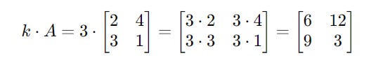
For example, for matrix A and scalar k as shown below:
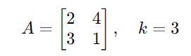
Scalar multiplication on these is shown below:
Matrix Multiplication
Two matrices can only be multiplied if the number of columns in the first matrix equals the number of rows in the second matrix.
Two matrices A and B:
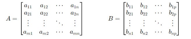
where:
A is a
m × nmatrixB is a
n × pmatrix
The resulting matrix C in this case, will be a m × p matrix.
The product of A and B is calculated using the formula:
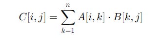
where:
C[i, j]is the element in thei-th row andj-th column of the resulting matrixC.A[i, k]is the element in thei-th row andk-th column of matrixA.B[k, j]is the element in thek-th row andj-th column of matrixB.The products of corresponding elements in the row of
Aand column ofBare summated to compute elements inC.
This process is much simplified in the illustration shown below.
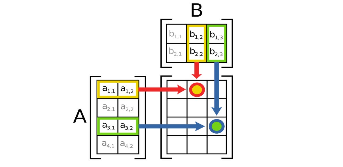
Let’s learn this using an example.
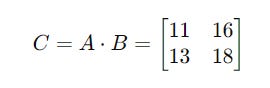
For matrices A and B shown below:
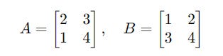
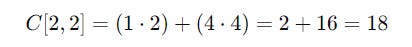
The resulting matrix C after multiplying them is the following:
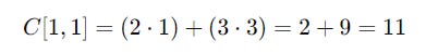
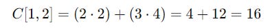
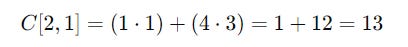
Each step in the calculation is shown below:
Tensor Product Of Matrices
The tensor product of two matrices is also called the Kronecker product.
Given two matrices A and B of size m × n and p × q respectively, their tensor product A ⊗ B results in a matrix of size (m ⋅ p) × (n ⋅ q).
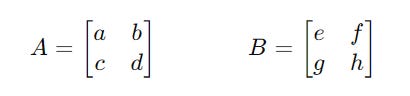
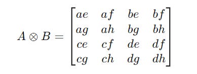
For two matrices A and B as shown below:
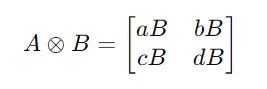
Their tensor product is calculated as follows:
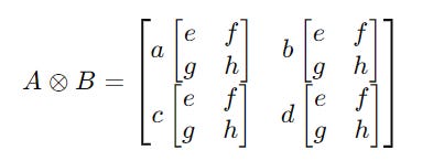
Expanding these gives:
In Quantum computing, the tensor product is used to:
Represent the state of a multi-qubit system
Represent Quantum gates
Identity Matrix
An Identity matrix is similar to 1.
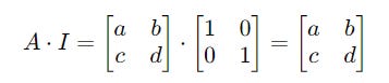
Similar to how multiplying a number by 1 leaves it unchanged, multiplying a matrix with its identity matrix leaves it unchanged.
Consider a matrix A and a 2 x 2 identity matrix I.
Multiplying A with I returns the same matrix A.
What Does An Identity Matrix Look Like?
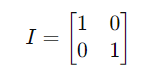
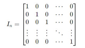
In an Identity matrix, all diagonal elements are 1, and all off-diagonal elements are 0.
A n x n identity matrix I(n) looks like the following:
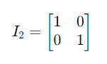
The 2 x 2 Identity matrix is:
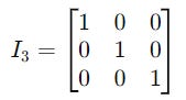
Similarly, the 3 x 3 Identity matrix is:
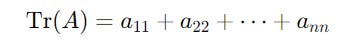
Trace Of A Matrix
For a square matrix, its Trace is the sum of its diagonal elements.
For a matrix A as shown below:
Its Trace is calculated as follows:
For a matrix A as follows:
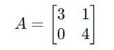
Its trace is 7 (the sum of its diagonal elements 3 and 4).
The Trace of a matrix is equal to the sum of its eigenvalues. (We will revisit this point in one of the following lessons.)
Determinant Of A Matrix
Determinant is a number that gives important information about a square matrix.
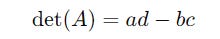
For a square matrix of dimensions 2 x 2 shown below:
Its determinant is calculated as:
For a square matrix of dimensions 3 x 3 shown below:
Its determinant is calculated as:

For larger matrices, the Leibniz formula can be used to calculate the determinant of an n x n matrix.
An important use case of the determinant is to find if a matrix has an inverse.
This is discussed in the next section.
Matrix Inversion
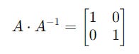
The inverse of a matrix A is a matrix that, when multiplied by the original matrix, yields the Identity matrix.
In other words, for a matrix A, its inverse A^-1 satisfies the following property:
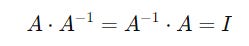
where I is the identity matrix.
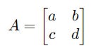
For a matrix A as shown below:
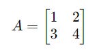
Its inverse is given by A^-1:
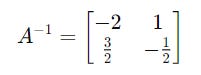
And they satisfy the following property:
Which Matrices Can Have An Inverse?
For a matrix to have an inverse:
It should be a Square matrix.
It should have a non-zero determinant.
If the determinant of a matrix is zero, it is a Singular matrix, or it has no inverse.
How To Calculate The Inverse Of A Matrix?
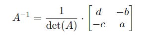
For a 2 x 2 matrix:
Its inverse is given by the following formula:
For larger matrices, the following methods can be considered:
Matrix Division
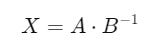
Matrices cannot be divided directly like numbers.
In other words, dividing a matrix by another matrix is an undefined function.
However, matrix division can be performed indirectly by multiplying one by the inverse of another matrix.
The lesson on Linear algebra is broken down into different parts to make it easy to learn.
Stay tuned for the next part!