How To Create Quantum Circuits With Qiskit

Solution to Question 1 and 2 of the ongoing Quantum programming challenge

Hey everyone!

Last week, I published a challenge with 6 Qiskit questions to get started with Quantum Computing.

6 Qiskit Questions to Get Started with Quantum Computing

Here are the solutions to the first two questions from the challenge.

---

Question 1

Create a 1-qubit quantum circuit that:

1. Starts in the state |0>

2. Applies a Hadamard gate

3. Measures the qubit

Write the Qiskit code and simulate the circuit using a Qiskit simulator.

---

Solution 1

We start by installing Qiskit and the Qiskit Aer library.

Qiskit Aer is a high-performance library with realistic noise models to run quantum computing simulations on classical computers.

!uv pip install qiskit qiskit-aer 

If you’re interested in running the following code on a real quantum computer, refer to the following article.

A Practical Guide To Running Your First Program On An IBM Quantum Computer

Next, we import the necessary packages.

from qiskit import QuantumCircuit # To create and manipulate quantum circuits

from qiskit_aer import Aer # Qiskit simulator backend 

from qiskit.visualization import plot_histogram # To visualise measurement results 

We then create the quantum circuit using QuantumCircuit(1, 1) where the:

• First 1 represents one qubit. This qubit is in state |0>.

• Second 1 represents one classical bit used to store the measurement result.

# Create circuit 
circuit = QuantumCircuit(1, 1) 

Next, we apply the Hadamard gate to the qubit and then measure it.

# Apply Hadamard gate to qubit at index 0
circuit.h(0) 

# Measure qubit at index 0 and store in classical bit at index 0
circuit.measure(0, 0) 

This is how these operations look.

# Visualise the circuit operations
print(circuit)

     ┌───┐┌─┐
  q: ┤ H ├┤M├
     └───┘└╥┘
c: 1/══════╩═
           0 

In the above circuit visualisation:

• the single horizontal line (-) represents the qubit connections

• the double line (═) represents the classical connections

• q represents the quantum register

• c: 1/ represents the classical register where measurement results are stored, where 1/ means that we have 1 classical bit

• ┤ H ├ is the Hadamard gate applied to the qubit

• ┤M├ is the Measurement operation

• ╩ is where the measurement result gets written to the classical bit

• 0 below the double lines indicates that the classical bit is at index 0

Now that we have created a quantum circuit, it is time to simulate it on the quantum simulator.

# Instantiate Qiskit quantum simulator
simulator = Aer.get_backend("qasm_simulator")

# Executes the circuit on the simulator for 1024 repetitions
job = simulator.run(circuit, shots = 1024) 

# Get the measurement results
result = job.result()
counts = result.get_counts(circuit)

print(counts)
# Output: {'0': 507, '1': 517}

We run the simulations for 1024 independent shots. This means that the circuit resets to |0>, applies an H gate, measures, and records the result. That’s why we get a distribution of outcomes rather than just one answer.

The counts value represents how many times each outcome occurred.

These outcomes are visualised as follows.

plot_histogram(counts)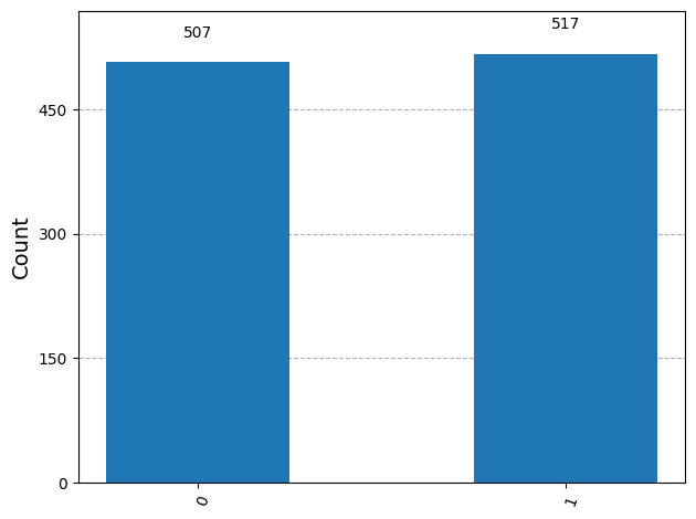

This is how we calculate the probabilities for each outcome.

# Calculate probabilities
total_shots = sum(counts.values())
for outcome, count in counts.items():
    probability = (count / total_shots) * 100
    print(f"|{outcome}⟩: {count} counts ({probability:.1f}%)")

"""
Output:
|0⟩: 507 counts (49.5%)
|1⟩: 517 counts (50.5%)
"""

To revise, the following operations take place in the above circuit:

• The qubit starts in the state |0>

• When the Hadamard gate is applied, it transforms the qubit into a quantum superposition (|0⟩ + |1⟩)/√2

  This means that the qubit simultaneously exists in both the |0⟩ and |1⟩ states with equal probability amplitudes.

• When we measure the qubit, this superposition instantly collapses to either |0⟩ or |1⟩, each with a 50% probability.

• Since we run the circuit 1024 times (shots), we observe approximately equal counts of “0” and “1”, confirming the equal superposition created by the Hadamard gate. With more shots, the counts would converge even closer to 50/50.

It’s time to move to solving question 2.

---

Question 2

Create a 1-qubit quantum circuit that:

1. Applies an X gate

2. Applies a Z gate

3. Measures the qubit

Write the Qiskit code and simulate the circuit using a Qiskit simulator.

---

Solution 2

from qiskit import QuantumCircuit
from qiskit_aer import Aer
from qiskit.visualization import plot_histogram

# Create circuit with 1 qubit and 1 classical bit
circuit = QuantumCircuit(1, 1)

# Apply X gate (flips |0> to |1>)
circuit.x(0)

# Apply Z gate (adds phase to |1>)
circuit.z(0)

# Measure qubit 0 and store in classical bit 0
circuit.measure(0, 0)

# Visualize the circuit
print(circuit)

     ┌───┐┌───┐┌─┐
  q: ┤ X ├┤ Z ├┤M├
     └───┘└───┘└╥┘
c: 1/═══════════╩═
                0

# Simulate
simulator = Aer.get_backend("qasm_simulator")
job = simulator.run(circuit, shots=1024)
result = job.result()
counts = result.get_counts(circuit)

print(counts) 
# Output: {'1': 1024}

# Calculate probabilities
total_shots = sum(counts.values())
for outcome, count in counts.items():
    probability = (count / total_shots) * 100
    print(f"|{outcome}⟩: {count} counts ({probability:.1f}%)")

# Output: |1⟩: 1024 counts (100.0%)

plot_histogram(counts)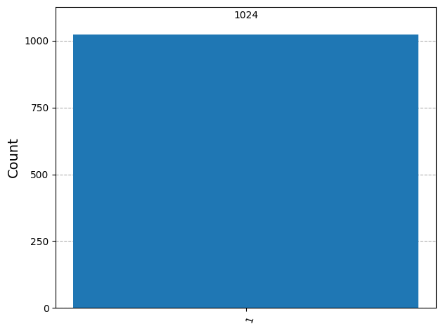

The following operations take place in the above circuit:

• The qubit starts in the state |0⟩

• When the X gate is applied, it flips the qubit: X|0⟩ = |1⟩.

• When the Z gate is applied, it adds a phase factor: Z|1⟩ = -|1⟩. This global phase doesn’t affect measurement outcomes in the computational basis.

• When we measure the qubit, it collapses to |1⟩ with 100% probability.

• Since we run the circuit 1024 times (shots), we observe all 1024 measurements as “1” and none as “0.”

---

That’s everything for this article.

Thanks for being a curious reader of ‘Into Quantum’, a publication that teaches essential concepts in Quantum Computing from the ground up.

To get even more value from this publication, consider becoming a paid subscriber.

See you soon in the next lesson.