An Introduction To Eigenvectors & Eigenvalues Towards Quantum Computing

Learn the mathematical basis of quantum measurements by performing them by hand.

Apr 04, 2025

Photograph of **David Hilbert**, an incredible mathematician who laid the theoretical groundwork for understanding eigenvalues and eigenvectors within quantum systems and the development of Hilbert space that provides the bedrock for quantum mechanics. (Source: Wikimedia Commons)

Eigenvectors & Eigenvalues are two important terms you will encounter multiple times when reading about Quantum Computing.

These terms are crucial to understand, and this lesson is all about them.

Let’s do this step by step.

Matrices

We start with Matrices that we have extensively discussed in a previous lesson.

A Matrix is a rectangular array of numbers (elements).

A m x n matrix has m rows and n columns.

For example, a 3 x 2 matrix is shown below:

Matrices are used to describe linear transformations between vectors.

Multiplying a matrix by a vector is equivalent to applying the linear transformation represented by that matrix to the vector.

Square Matrix

A matrix with the same number of rows and columns is called a Square matrix.

A 3 x 3 square matrix is shown below:

Identity Matrix

An identity matrix is a type of square matrix that acts like the number 1 in matrix multiplication.

Any matrix, multiplied by an identity matrix I of the same size, leaves it unchanged.

Eigenvector

Given a square matrix A of size n x n, an eigenvector is a non-zero vector v that, when multiplied by A, results in a scalar multiple of itself.

Eigenvectors multiplied with A just stretches or compresses them without rotation or change in direction.

Eigenvalue

The scalar in the above-described operations is called the eigenvalue, and it is denoted λ.

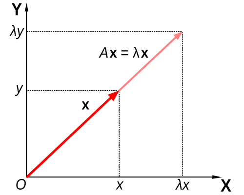
Eigenvalue λ represents how much the eigenvector v is scaled (stretched or shrunk) by the transformation defined by matrix A.

This is shown mathematically as follows:

where:

A is the matrix (representing a linear transformation)
v is the eigenvector of matrix A
λ is the eigenvalue of matrix A

This concept is further explained with the plot below.

Matrix A acts by stretching the vector x (not changing its direction), so x is an eigenvector of A. (Source: Wikimedia Commons)

(For the interested ones, the word “eigen” comes from German and means “own” or “characteristic.”)

How To Find Eigenvalues?

To find eigenvalues of a matrix, we solve the following equation (called the characteristic equation of matrix A).

where:

A is the square matrix with dimensions n x n
I is the Identity matrix
λ is the eigenvalue (that we need to calculate)
det is the determinant function

This solution gives us a polynomial equation in terms of λ called the characteristic polynomial.

The roots of this polynomial (value of λ where the polynomial equals 0) are the eigenvalues of A.
The degree of the polynomial (highest power of λ in the polynomial) equals the size of the A.

How To Find Eigenvectors?

For each eigenvalue, we find the corresponding eigenvectors by solving:

This equation is derived by rearranging the following equation:

where I is the Identity matrix, so λIv = λv.

We multiply λ by the identity matrix I because it turns the scalar λ into a n × n matrix (λI), which can now be subtracted from A.

Calculating Eigenvalues and Eigenvectors: A Practical Example

Consider a 2 x 2 square matrix A:

To find the eigenvalues associated with it, we solve the characteristic equation:

Let’s solve this step by step.

We first calculate the term λI as follows:

Next,

The determinant of a 2 x 2 matrix can be calculated using the formula:

where:

Using this:

Plugging this term into the characteristic equation gives us the following quadratic equation:

Solving this using the Quadratic formula returns the following eigenvalues:

Let’s calculate the eigenvectors associated with these eigenvalues, using the following equation:

For λ = 5:

Putting this in the equation returns:

So the associated eigenvector with eigenvalue 5 is:

For λ = 2:

Putting this in the equation returns:

So the associated eigenvector with eigenvalue 2 is:

Why Are We Interested In These?

Here’s the reason.

In quantum mechanics, matrices are used as Operators.

Operators are mathematical transformations that act on a quantum state to produce another quantum state.

Every measurable quantity (called an Observable) is represented by a Hermitian operator (Â) (a square matrix equal to its conjugate transpose).

where † represents the Conjugate transpose/ Hermitian adjoint operation.

When we measure this observable (by applying the corresponding operator), we get one of its eigenvalues λ(i), and the system collapses into the corresponding eigenvector |a(i)>.

The eigenvalues are the measurement outcomes, and the corresponding eigenvectors are states the system will be in after the measurement.

Mathematically:

where:

Â is an observable, represented by a Hermitian operator.
|a(i)> is an eigenvector of Â. It is also called the eigenstate of Â in quantum mechanics.
λ(i) is the eigenvalue (a real number) corresponding to the eigenvector |a(i)>

But why use Hermitian operators to represent observables?

This is because:

Hermitian operators have real eigenvalues

Since an observable (position, momentum, energy, etc) must return real-valued results when measured, Hermitian operators are the perfect fit.

If observables weren’t Hermitian, measurements could return complex numbers, which wouldn’t correspond to physically meaningful measurements.

2. Eigenvectors corresponding to distinct eigenvalues of Hermitian operators are Orthogonal

On measurement, a system moves into one of the eigenvectors of the observable’s operator.

Since the eigenvectors for different eigenvalues are orthonormal, they form the basis in the Hilbert space and span the space.

What Happens When A Measurement Is Done?

Any quantum system |ψ> can be represented as a superposition of eigenvectors/ eigenstates of Â:

where c(i) is the Probability amplitude associated with each eigenvector/ eigenstate |a(i)>.

Post measurement, the probability of obtaining the result λ(k) (one of the eigenvalues) is:

And after the measurement result λ(k), the system collapses into one of the eigenvectors/ eigenstates, randomly:

If the measurement is performed multiple times, we can find the average value of the results (also known as the Expectation value) by the following equation:

Let’s understand this in depth using a practical example.

In Quantum computing, the Pauli-Z operator (Ẑ) measures the spin along the z-axis in the Bloch sphere representation.

It is Hermitian because it is equal to its own conjugate transpose.

Ẑ has two eigenvectors:

which corresponds to the eigenvalue of +1.

And,

which corresponds to the eigenvalue of -1.

Following the equation,

What we discussed can be written as:

These eigenvectors/ eigenstates |0> and |1> form an eigenbasis for the Pauli Z matrix.

These eigenvectors/ eigenstates are also the computational basis states used in quantum computing, where:

|0> represents Spin up along the z-axis, or classical bit 0
|1> represents Spin down along the z-axis, or classical bit 1

Calculating Eigenvectors And Eigenvalues Of `Ẑ`

We know that Ẑ is a Hermitian operator as shown below:

Coming back to the characteristic equation:

Let’s calculate the inner term:

And then it's determinant:

These are the eigenvalues of Ẑ.

Using the equation:

where:

For λ = 1:

Putting this term in the equation:

This gives y = 0.

Since x is a free term, we pick it as 1 and the eigenvector associated with the eigenvalue +1 is:

Similarly, for λ = -1, we start from:

Next, we find the term:

Putting this term in the equation:

This gives x = 0.

Since y is a free term, we pick it as 1 and the eigenvector associated with the eigenvalue –1 is:

We pick 1 for the free values in these eigenvectors because it makes the vector representation simple by normalising them (having a unit length).

Performing Measurements And Calculating Expectation Value

Let’s say that a quantum system representing a qubit is in a state of equal superposition like the following:

Measuring them using the Pauli-Z operator will return the eigenvalues with a 50% probability for each, and once measured, the system will be out of superposition and in the respective eigenvector/ eigenstate.

Let’s calculate the expectation value or the average value of the results obtained from measuring Ẑ (spin in Z-axis) on many systems prepared in the state ∣ψ>.

We know that initially our quantum system is in the state represented by the ket vector |ψ>: