All The Math That You Need To Start Doing Quantum Computing (Part-3)
Lesson 3: Differential Calculus

Here’s the third part of the series that introduces all the mathematics you must understand to start doing quantum mechanics and quantum computing.
Here are the previous ones, in case you missed them:
Lesson 3: Differential Calculus
Limit
Let’s say that we have a sequence of numbers that reach close to a particular value.
For example:
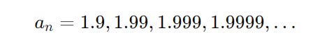
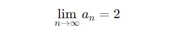
The limit of this sequence is 2, as n approaches infinity (n → ∞).
It is written as:
Similarly, for a function, the limit describes the value that the function approaches as its input approaches a particular point.
It is written as:
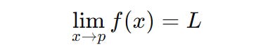
For the above, L is the limit of f(x) as x approaches p.
Or, f(x) tends to L as x tends to p.

Derivatives
Differential Calculus is used to study quantities that change smoothly or continuously.
It is applied to evaluate the rate of change of such quantities.
Consider a function called f(x).
Let’s observe how it changes as we change x. This change is Δx.
Note that the Δ symbol represents a change in a quantity.
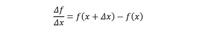
If we want to get more precise at evaluating Δf (the change in f) with respect to Δx, we need to let Δx get as close to 0 as possible.
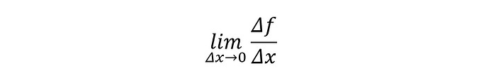
This limit is called the Derivative of the function f(x) with respect to x.
This is written as:
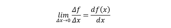
or,
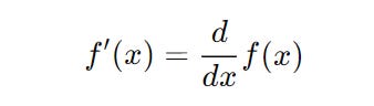
where d represents Δ with the limit approaching zero.
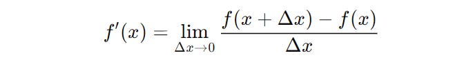
The derivative of a function of x or f(x) with respect to x can be calculated as follows:
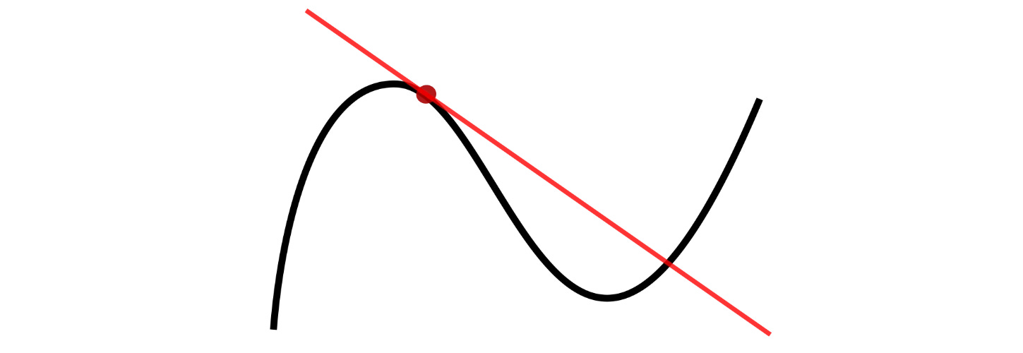
It is interesting to note that the slope of the tangent line to the curve y = f(x) at a specific point is the derivative of the function f(x) at that point.
Rules Of Differential Calculus
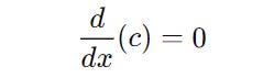
Constant Rule
The derivative of a constant is always zero.
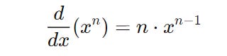
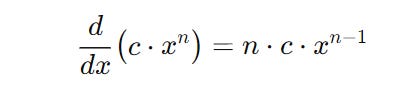
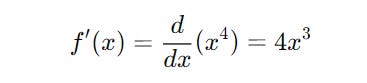
Power Rule
For a function of the form f(x) = x^n its derivative is given as follows.
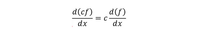
Constant Multiple Rule
Derivative of constant times a function is constant times the derivative of the function.
Note how the following derivative is calculated using the power rule and the constant multiple rule:
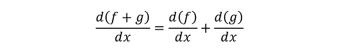
Sum Rule
For two functions of x i.e. f(x) and g(x), the derivative of their sum is calculated as below:
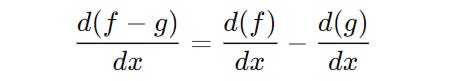
Difference Rule
For two functions of x i.e. f(x) and g(x), the derivative of their difference is calculated as below:
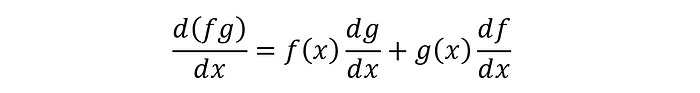
Product Rule
For two functions of x i.e. f(x) and g(x), the derivative of their product is calculated as below:
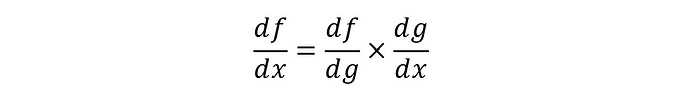
Chain Rule
For a function of x i.e. g(x) and another function of g i.e. f(g), derivative f(g) with respect to x is calculated as follows:
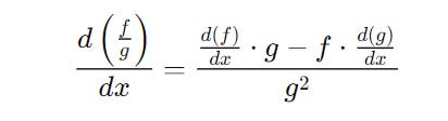
Quotient Rule
If f(x) and g(x) are two functions, the derivative of their quotient is calculated as follows:
Commonly Used Derivatives
Some commonly used derivatives are as follows:
d(x)/dx = 1d(e^x)/dx = e^x, whereeis Euler’s number (e ≈ 2.718)d(ln x)/dx = 1/x, wherelnis the natural logarithmd(sin x)/dx = cos xd(cos x)/dx = — sin xd(tan x)/dx = sec^2 x
Higher-Order Derivatives
A higher-order derivative is a derivative of a derivative.
In other words, it is the rate of change of the previous derivative.
If f′(x) is the first derivative of the function f(x), then:
The derivative of
f′(x)is called the second derivative.It is denoted as
f′′(x).The derivative of
f′′(x)is called the third derivative.It is denoted in the following example.
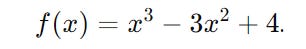
For a given function:
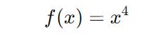
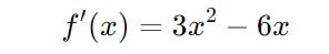
Its first derivative is:
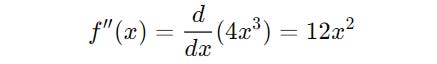
Its second derivative is:
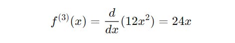
And its third derivative is (and so on):
Finding Maxima And Minima Of A Function
Finding the best possible outcome (maximum/ maxima or minimum/ minima) of a function in a given context is called Optimization.

The steps for finding the maxima and minima are as follows.
Step 1: Find the First Derivative
This is the slope of the curve of the function.
Step 2: Find the Critical Points
In this step, we first set the first derivative to zero to find the points where the slope is flat.
Next, we solve for x. The values obtained are the critical (flat slope) points where the curve could have its maxima or minima.
Step 3: Test the Critical Points
In this step, we calculate the second derivative of the function.
Three possibilities arise here:
If the second derivative is greater than 0, the curve is concave up, and the critical point is a minima.
If the second derivative is less than 0, the curve is concave down, and the critical point is a maxima.
If the second derivative is 0, the test is inconclusive.
Let’s find the maxima and minima of the following function:
Step 1 is finding its first derivative.
Step 2 is to find the critical points by setting f’(x) to 0.

Step 3 tests these critical points by calculating the second derivative.
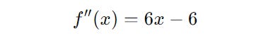
For x = 0 :
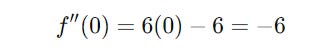
As this result is less than 0, the function has its maximum at x = 0.
For x = 2 :
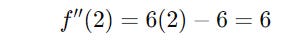
As this result is greater than 0, the function has its minimum at x = 2.
We can substitute the values of x into the original function to find the y coordinates of the maxima and minima.
This list of concepts in Differential Calculus is not exhaustive, but good enough to start with.
See you soon in the next part.